
K-Means 101
K-Means 101
I’ve been working a lot with the Museum of Modern Art’s collection dataset recently and thought it would be useful to cluster paintings based on size.
One approach would be to use pandas.cut() or pandas.qcut() to choose cutoff points for small, medium, and large works, but this would require choosing only one of the size features that we have: either Width (cm), Height (cm), or my engineered feature of Area (cm sq). Perhaps using Area (cm sq) would give us a good approximation, but there’s another problem: how many segments do we want? Here I suggested three–small, medium, and large–but this decision is somewhat arbitrary. Why not 4? 5? More?
An alternative approach is to use a clustering algorithm to cluster the data based on all three size features, and then using the ‘elbow method’ to find the optimal number of clusters. That’s what I’ll do here.
A Brief Overview of the Data
Before proceeding, let’s check in with the dataset and remind ourself what the size features look like.
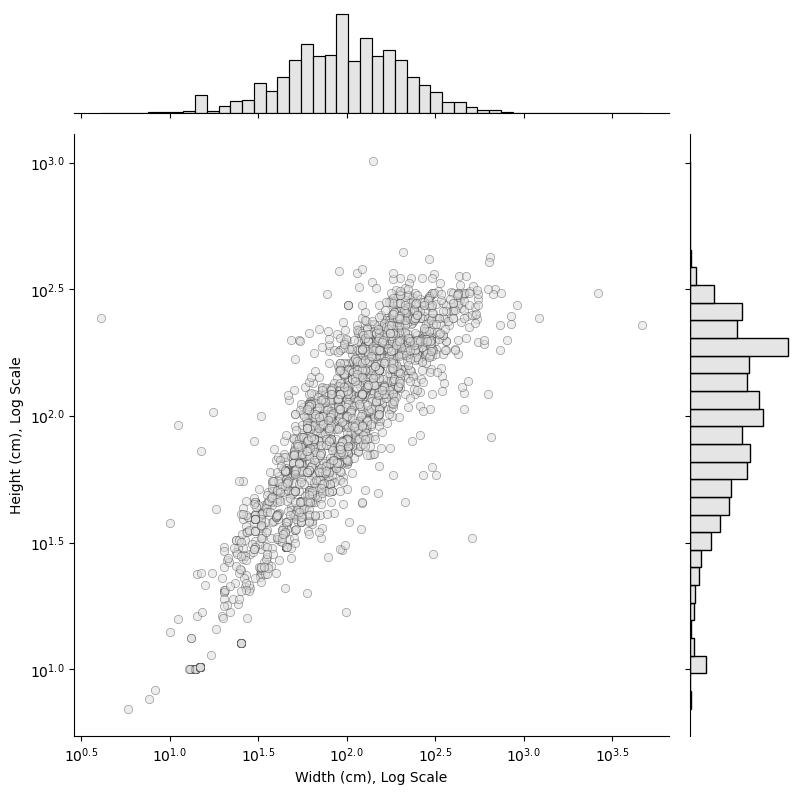
Here I’m just plotting height and width, of course. What we see is that painting size, when plotted on a logarithmic scale, forms a mostly continuous and normal distribution. Obviously we’re missing the Area (cm sq) feature here, but judging by Height (cm) and Width (cm) it isn’t really obvious how many clusters there ought to be, nor where their boundaries are.
This is where K-Means can help us.
Using K-Means
Implementing K-Means is super easy. First I’m going to isolate the features of interest–Width (cm), Height (cm), and Area (cm sq). Then I’ll run the clustering algorithm multiple times with varying numbers of clusters.
X = np.log10(paintings[['Width (cm)', 'Height (cm)', 'Area (cm sq)']])

# Cluster trying k = 1-10
k_values = []
inertia_values = []

for k in range(1, 11):
    kmeans = KMeans(n_clusters=k, random_state=0).fit(X)
    k_values.append(k)
    inertia_values.append(kmeans.inertia_)
If we plot the result, we can see the inertia score (lower is better) as a function of the number of clusters.
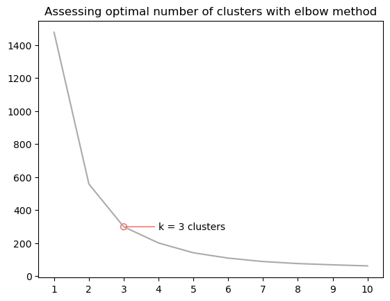
As to be expected, the fit improves as the number of clusters k increases, but the rate of improvement decreases substantially after k = 3 clusters. Here’s the ‘elbow method’ in action. Turns out 3 clusters–small, medium, and large–fits the data pretty well, so we’ll stick with that.
Visualizing the Result
Let’s have another look at the scatter plot (again, just width and height features), but with our new clusters colod-coded.
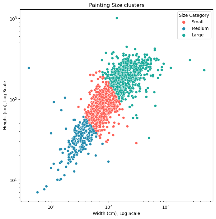
There you have it! Now we can use this new categorical feature that I’ve created to segment the data in new ways.