Art Auction Data: Exploratory Data Analysis, Andy Warhol Case Study, Part II: NLP

A series of posts related to an art auction price model project.

Case Study of Andy Warhol, Part II: Adding NLP Features

In my previous notebook I developed some good intuition for Warhol’s market and for some of the features that correlate with price.

Warhol (okay, not quite, but good enough) presenting charts and graphs, created by Midjourney

However, one glaring omission was the two messy text fields: artwork title and medium. At first it might not seem obvious how these fields would correlate with price, but I have some hypotheses:

• Keywords found in the title will, in Warhol’s case specifically, function as proxies for various bodies of work. For example, Warhol made Elvis works only briefly, so the keyword elvis should help to identify a certain body of work and capture something of that body of work’s significance, its scarcity, and its market dynamics. Whereas works related to Marilyn Monroe or Jacqueline Onassis have their own unique date spans and help to identify different bodies of (variously) related work. Essentially I am expecting that title keywords, in Warhol’s case, should help cluster similar works together in a way that makes it easier for the algorithm.
• Title keywords should capture demand for certain types of content. In addition to helping identify specific bodies of work, I suspet that title keyworks will also make it possible to see patterns in demand for certain kinds of content. In instances where Warhol worked with a similar motif over a long period of time, for example, a title keyword may be less effective at identifying a narrow body of historically related work than identifying subject matter, and perhaps some subject matter is more popular than others (again, not for historical reasons but because of trends in collecting or personal taste, etc).
• Medium keywords will help parse an otherwise messy feature. The medium feature is particularly knotty, so doing some rudimentary vectorization of its component words should offer a way of grouping things into particular categories. Knowing whether a work was a screenprint or a scrulpture or a polaroid or a drawing will presumably be very important in predicting its market value.

Medium

Let’s start with medium. To get a rough sense of what we’re dealing with here, I’ll make a wordcloud.

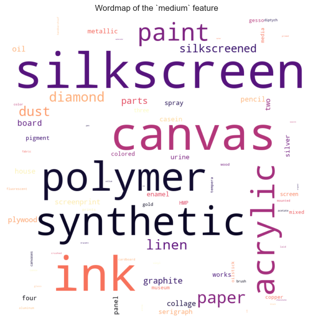
This wordcloud gives us a very quick and dirty sense of what words come up most often in the medium feature.

The WordCloud object has a words_ attribute, which is a dictionary of the above word tokens and their associated frequency. It would not be complicated to loop through that list and look at price distributions for titles containing each of those tokens. However, vectorizing this feature using sklearn.feature_extraction.text.CountVectorizer will ultimately provide an easier way of doing this.

But before doing that, notice that there are some similar words in the wordcloud: ‘silkscreen’, ‘silkscreened’, and ‘screenprint’, for example. I think it’s safe to assume that these are referring to the same thing and should be merged. I considered using a stemmer such as nltk.stem.snowball.SnowballStemmer to reduce words to common stems, however this wouldn’t capture a discrepancy like ‘silkscreen’ and ‘screenprint.’

New plan:

• I’ll do a pass with sklearn.feature_extraction.text.CountVectorizer (no stopwords) and get a list of all the word tokens found in the medium feature
• I’ll import these words into OpenRefine, which has some good clustering support to find similar words
• With the results, I’ll find and replace old words (e.g., ‘screenprint’, ‘silkscreen’, ‘silkscreened’) with a normalized word (‘silkscreen’)
• Then, I’ll use the CountVectorizer on the new, normalized medium feature to extract tokens.

# Instantiate CountVectorizer object
countvectorizer = CountVectorizer(
    analyzer='word',
)

# Fit vectorizer
count_wm = countvectorizer.fit_transform(warhol['medium'].fillna(''))

# Convert to DataFrame
medium_tokens = pd.DataFrame(data=count_wm.toarray(), columns=countvectorizer.get_feature_names_out())

medium_tokens.head()

	10	16	acetate	acrylic	aid	album	aluminum	and	aniline	appliqué	...	watermarked	white	whitman	with	wood	works	wove	wrapped	wrapping	yellow
0	0	0	0	0	0	0	0	0	0	0	...	0	0	0	0	0	0	0	0	0	0
1	0	0	0	0	0	0	0	0	0	0	...	0	0	0	0	0	0	0	0	0	0
2	0	0	0	1	0	0	0	1	0	0	...	0	0	0	0	0	0	0	0	0	0
3	0	0	0	0	0	0	0	0	0	0	...	0	0	0	0	0	0	0	0	0	0
4	0	0	0	1	0	0	0	1	0	0	...	0	0	0	0	0	0	0	0	0	0

5 rows × 220 columns

Above is what the first pass of the medium field looks like: a sparse matrix comprising 250 keyword tokens as feature names and values indicating the occurrence of each token in each work.

Let’s have a look at the most frequently-occurring tokens:

# Count up occurrences of each token and preview
tokens_sum = medium_tokens.sum().sort_values(ascending=False)
tokens_sum.head(10)

on            2532
silkscreen    2344
and           2305
canvas        2102
ink           1664
polymer       1524
synthetic     1495
acrylic        933
inks           548
paint          478
dtype: int64

Notice that we’re getting keywords that are typically excluded–things like ‘on’ or ‘and’. This is because I decided not to include stop words when instantiating the CounterVectorizer object, since 250 is not too many words to review and I didn’t want to miss anything important that might have been mistakenly excluded as a stopword.

At this point what I’ve decided to do is use OpenRefine to merge similar tokens, since tokens like silkscreen and screenprint and screenprinted should all be the same. Here’s the result:

	medium	medium_reduced
5198	synthetic polymer paint and silkscreen ink	synthetic polymer paint and silkscreen ink
2575	acrylic and silkscreen ink on canvas	acrylic and silkscreen ink on canvas
2197	acrylic and silkscreen ink on canvas	acrylic and silkscreen ink on canvas
3407	synthetic polymer and silkscreen ink on canvas	synthetic polymer and silkscreen ink on canvas
5660	synthetic polymer silkscreen	synthetic polymer silkscreen
3939	silkscreen ink on paper	silkscreen ink on paper
2348	acrylic and silkscreen ink on canvas	acrylic and silkscreen ink on canvas
4064	synthetic polymer and silkscreen ink on canvas	synthetic polymer and silkscreen ink on canvas
5193	synthetic polymer and silkscreen inks	synthetic polymer and silkscreen ink
2737	synthetic polymer paint and silkscreen ink on ...	synthetic polymer paint and silkscreen ink on ...

We can already get a rough sense for the way in which the medium feature has been reduced. Now let’s tokenize medium_reduced, join the result with our existing DataFrame, and visualize the price distributions vs. each token.

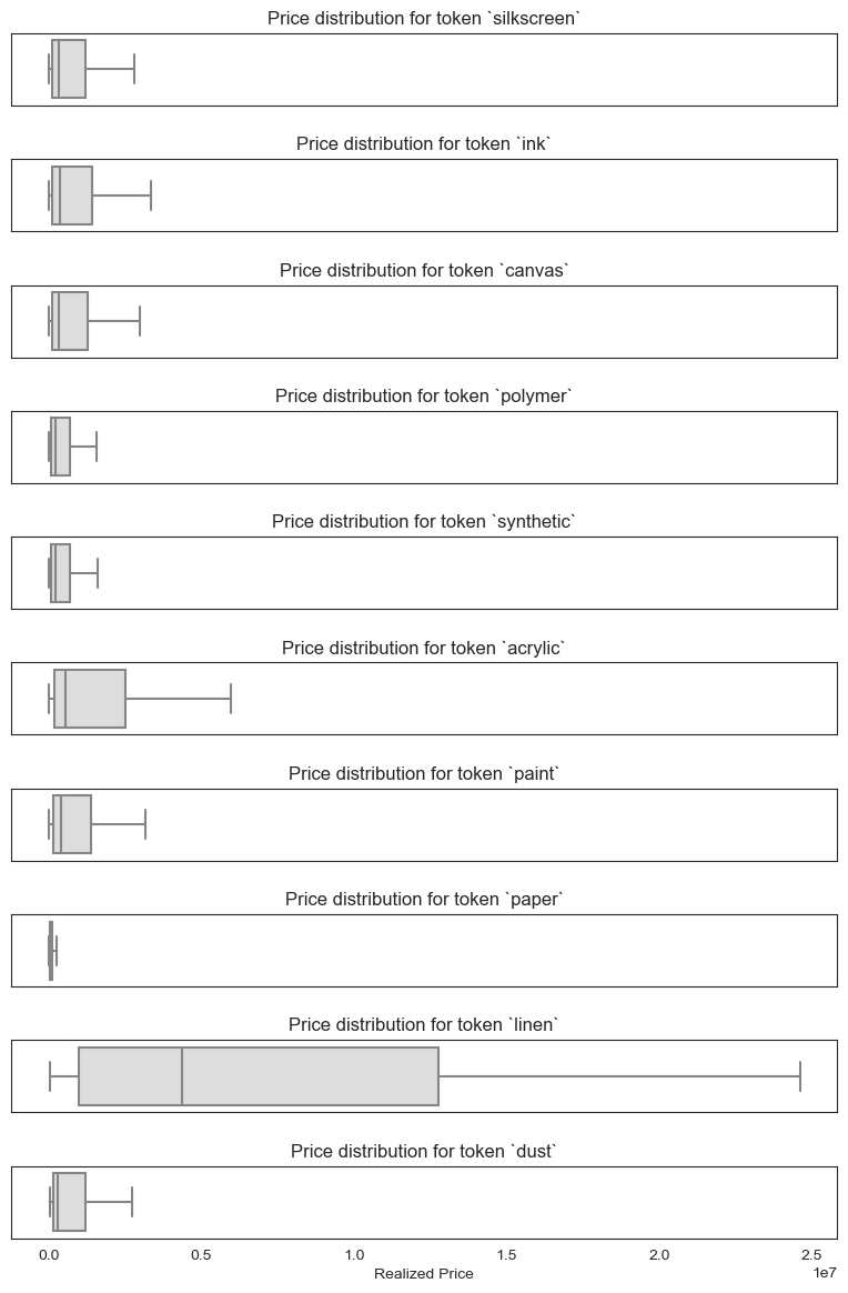
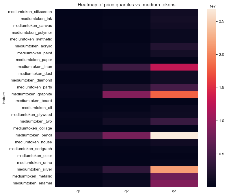
Interestingly we can see that some features of the medium column–namely keywords like ‘linen’, ‘graphite’, ‘pencil’, ‘silver’, and ‘enamel’–are associated with higher prices.

Engineering Features from title

Now we’ll do the same series of steps for the title feature.

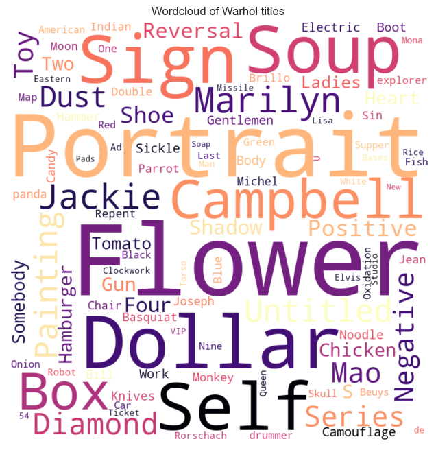
As with the medium wordcloud, this one gives us a fast sense of what Warhol’s titles look like in the context of this dataset.

There’s way more variability in the title feature than medium in terms of the sheer number of words, however. As a result, this time around I am going to use stop words and limit the number of features to 30 and we’ll go from there.

Let’s have a look at the most frequently-occurring tokens:

# Count up occurrences of each token and preview
tokens_sum = title_tokens.sum().sort_values(ascending=False)
tokens_sum

title_flowers      250
title_portrait     203
title_dollar       142
title_soup         118
title_self         115
title_sign         114
title_campbell     114
title_box          105
title_jackie        81
title_untitled      77
title_diamond       70
title_painting      65
title_dust          64
title_series        62
title_mao           60
title_marilyn       60
title_negative      58
title_positive      57
title_toy           55
title_reversal      50
title_four          48
title_shoes         46
title_marilyns      41
title_shadow        39
title_can           39
title_two           36
title_chicken       35
title_somebody      34
title_hamburger     34
title_ladies        31
dtype: int64

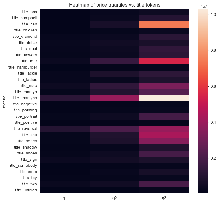
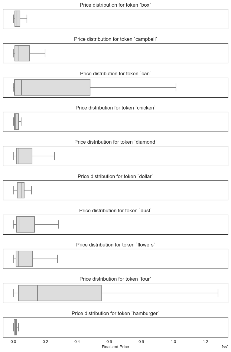
Even more so than with the medium feature, realized prices seem to vary significantly by title tokens–makes sense.

Tech:

Python Pandas Matplotlib Seaborn NumPy WordCloud Scikit-learn sklearn.feature_extraction.text.CountVectorizer

GitHub Repo