Art Stats Illustrated: Measures of Central Tendency
In this series of posts, I illustrate the fundamental stats concepts I'm teaching myself with art-related datasets.
What’s a Central Tendency?
One of the fundamental things we can do using statistics is summarize a whole bunch of values with a single number. What we’re interested in is a number that is representative of the larger set, a number that’s typical or average. In other words, a number that speaks to a central tendency.
There are a few ways of computing such a number, which you probably remember from high school:
- mean: the simple arithmetic mean of the numbers in your sample
- median: the halfway point in your sample–50% of the numbers are larger and 50% smaller
- mode: the most frequently-occurring value in the set.
I’m going to illustrate each of these, as well as go into more detail about when you’d use one over the other, using The Museum of Modern Art (MoMA) Collection Dataset, which, just like it sounds, contains information about all of the ~140,000 works in the museum’s collection. I’ve already cleaned and prepared this dataset for our purposes, too. To simplify the dataset, I’m going to focus on the 2,384 paintings in MoMA’s collection (or artworks classified as paintings, anyway), since that’s a relatively straightforward category and usually doesn’t involve complicated considerations–multiple artists, for instance, or complex date ranges.
The questions in particular that I’m going to examine and illustrate with these various measures of central tendency are as follows:
- For painters who were alive at the time of acquisition, how old did those artists tend to be?
- For painters who were no longer living at the time of acquisition, on the other hand, how many years after that artist’s death did the museum tend to wait?
- And regardless of whether or not the artist was alive at the time of acquisition, how old were their paintings when acquired?
By looking for typical values for these questions, we stand to learn something about the museum’s acquisition practices.
Mean vs. Median
Let’s start by computing the mean for a simple example. I’ll use a numpy method to do this, but the computation is simple: sum all the values and divide by the number of values.
# Import numpy
import numpy as np

# Set random seed for reproducibility
np.random.seed(123)

# Generate array of 10 integers from 0 to 10
arr = np.random.randint(0, 10, 10) # -> array([2, 2, 6, 1, 3, 9, 6, 1, 0, 1])

# Compute mean
np.mean(arr) # -> 3.1
Given that our array has several smaller numbers, a mean of 3.1 looks about right and seems pretty “typical” for the group.
To compute median, on the other hand, you sort your array and then select the middle item. In the case of even-numbered lists, you take the mean of the middle two numbers.
# Sort distribution
arr.sort() # -> array([0, 1, 1, 1, 2, 2, 3, 6, 6, 9])

# Compute median
np.median(arr) # -> 2.0
In this example, we have ten values, so we’d need to take the mean of the 5th and 6th values (i.e., 2 and 2), which is 2.
In this case, both 3.1 (the mean) and 2 (the median) seem like reasonable estimates of a central tendency. But what happens if the largest value is not 9 but 900?
# Increase largest value
arr[-1] = 900 # -> array([0, 1, 1, 1, 2, 2, 3, 6, 6, 900])

np.mean(arr) # -> 102.2

np.median(arr) # -> 2.0
What you can immediately see is that the new outlier value of 900 dramatically pulls the mean in that direction so that the mean is now 102.2! But since the median is concerned with the value at the 50th percentile, it remains the same. This is why we describe the median as “robust”: it is not vulnerable to extreme values in the way that the mean is. In this particular case, it’s obvious that 2.0 is a much better estimate of central tendecy than 102.2, which doesn’t describe the set of numbers we’ve been given very well at all.
Using Mean to Eestimate Painter’s Age at Acquisition
Let’s look at how old painters tend to be when their work is acquired. (Obviously this applies only painters who were living at that point in time.)
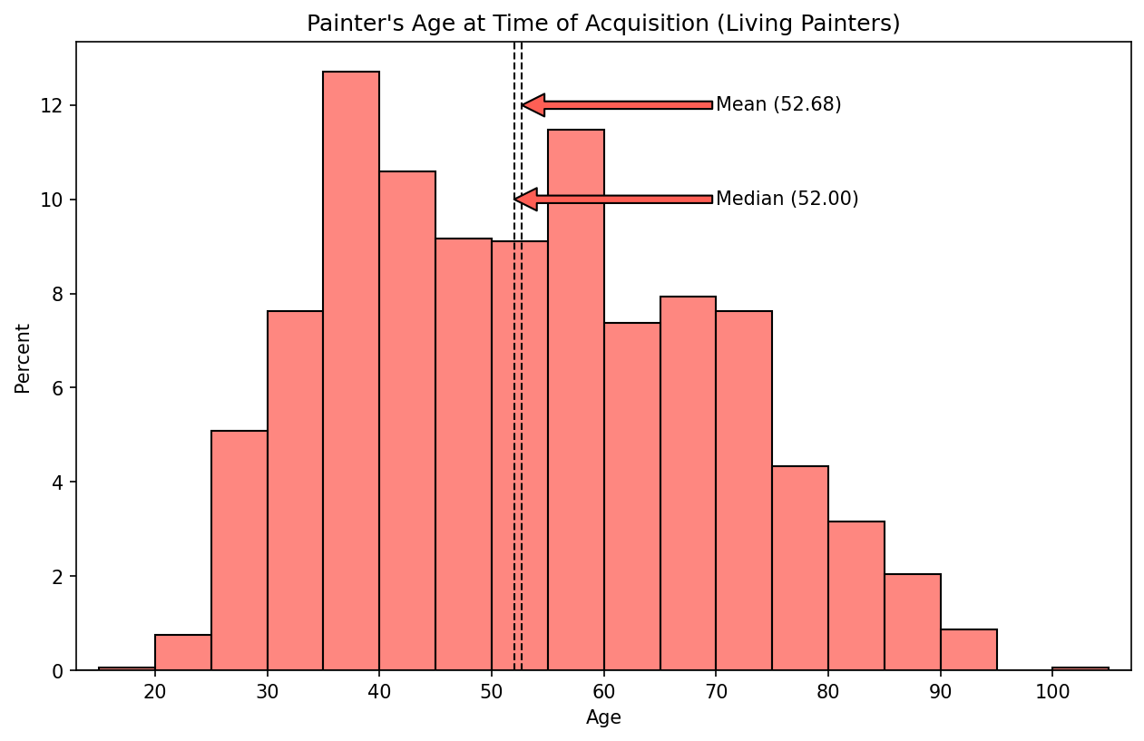
While visually it looks like there’s too much variance for this sample to resemble a normal distribution (more on that in another post), this distribution certainly looks pretty symmetrical. As a result, one of the things we see is that the mean and median are very close. The mean age of a painter at the time his/her work was acquired by MoMA is 52.68 years old, and the median is 52 years old. This is an example where the simple mean does a pretty good job of representing the overall numbers and allows us to say that painters who are still living tend to be later career when their work is acquired.
(And that’s interesting by the way! This gives us some indication of the museum’s conservatism or risk aversion: when it buys paintings from living artists, it privileges work by those who have been working for 30+ years–much “safer” for an institution invested in the history of art to collect paintings by artists whose legacy is already well-established.)
Using Median to Estimate Years Elapsed from Artist’s Death to Acquisition
For artists who were no longer living at the time their work was acquired, how much time has typically elapsed after the artist’s death until the work’s acquisition?
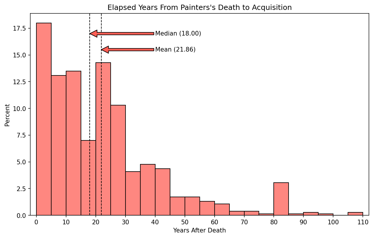
This is a very different-looking distribution, one that we’d describe as positively skewed, meaning that it has a tail to the right which has the effect of pulling the mean in the positive direction. Here the mean number of years after an artist has passed until the museum acquires a painting is 21.86 years. The median value, however, is 18 years.
Now, we can see by looking at this that there are very few examples of paintings that were acquired 70, 80, 90, 100 years after an artist has died. In fact, it’s quite common for paintings to be acquired not long after an artist’s death: about 17.5% of such acquisitions occur within 5 years, about 30% within 10, about 43% within 15. And actually, since the median is the value that’s exactly at thd halfway point, we can say definitively that 50% of all painting acquisitions made after the artist’s death occurred within 18 years, whereas the other half of such acquisitions fall somewhere between 18 and 110 years.
Because of this clustering of values on the left, the median would be a better and more robust representation of the central tendency here–robust meaning that it is less vulnerable to the outliers that we see on the right-hand side of the distribution, which, unlike the median, bias the mean in their direction. One can imagine an extreme scenario where MoMA, for some reason, acquires a medieval altarpiece–1,000 years, let’s say, after the artist’s death. This new datapoint would pull the mean up even higher, whereas the median would stay right where it is.
More Illustrations of Mean and Median: Artwork Age at Acquisition
I was also curious to look at artwork age at the time of acquisition–how new or old do paintings tend to be (that is, how many years after they were completed) when the museum buys them?
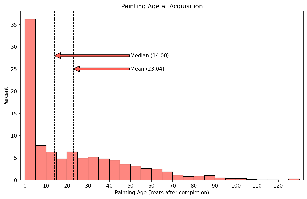
This is an even more positively skewed distribution than the last one. 35% of the time, paintings are less than 5 years old when acquired–that’s pretty new! And because the median is 14 years, we can say that half the time paintings are less than 14 years old when acquired. The other half of the time they’re somewhere between 14 and 130 years old. Because of the positive skew, the mean painting age is 23 years, which is clearly a less effective value for representing the central tendency here.
This is an interesting counterpoint to the artist age chart above, since it suggests that even while the museum tended toward conservatism in purchasing works from well-established, mid- to -late career artists, it also focused on new works. Which makes sense, as well: Once an artist and his/her legacy is established, then it’s safe to expand the collection with new and recent works.
As one final question, let’s see how this question of artwork age breaks down by whether or not the artist was alive at the time of acquisition.
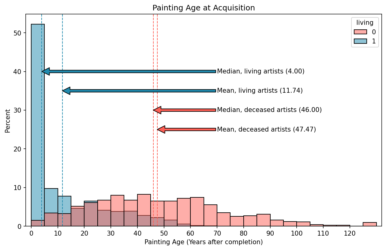
This is interesting to see, and intuitive, too.
For artists still living at the time of acquisition, the majority of paintings were acquired right away–looks like about 60% of paintings within 10 years. Here the positive skew is even more extreme, with a median time of 4 years but a mean time of nearly 12.
For artists who were no longer alive at the time of acquisition, the distribution is much more symmetrical, with a median time of 46 years and a mean time of 47.5. This distribution is pretty intuitive, as well, since the work of artists who are no longer of living will, by necessity, be older. Nevertheless, it’s curious to see just how much older the work tends to be.
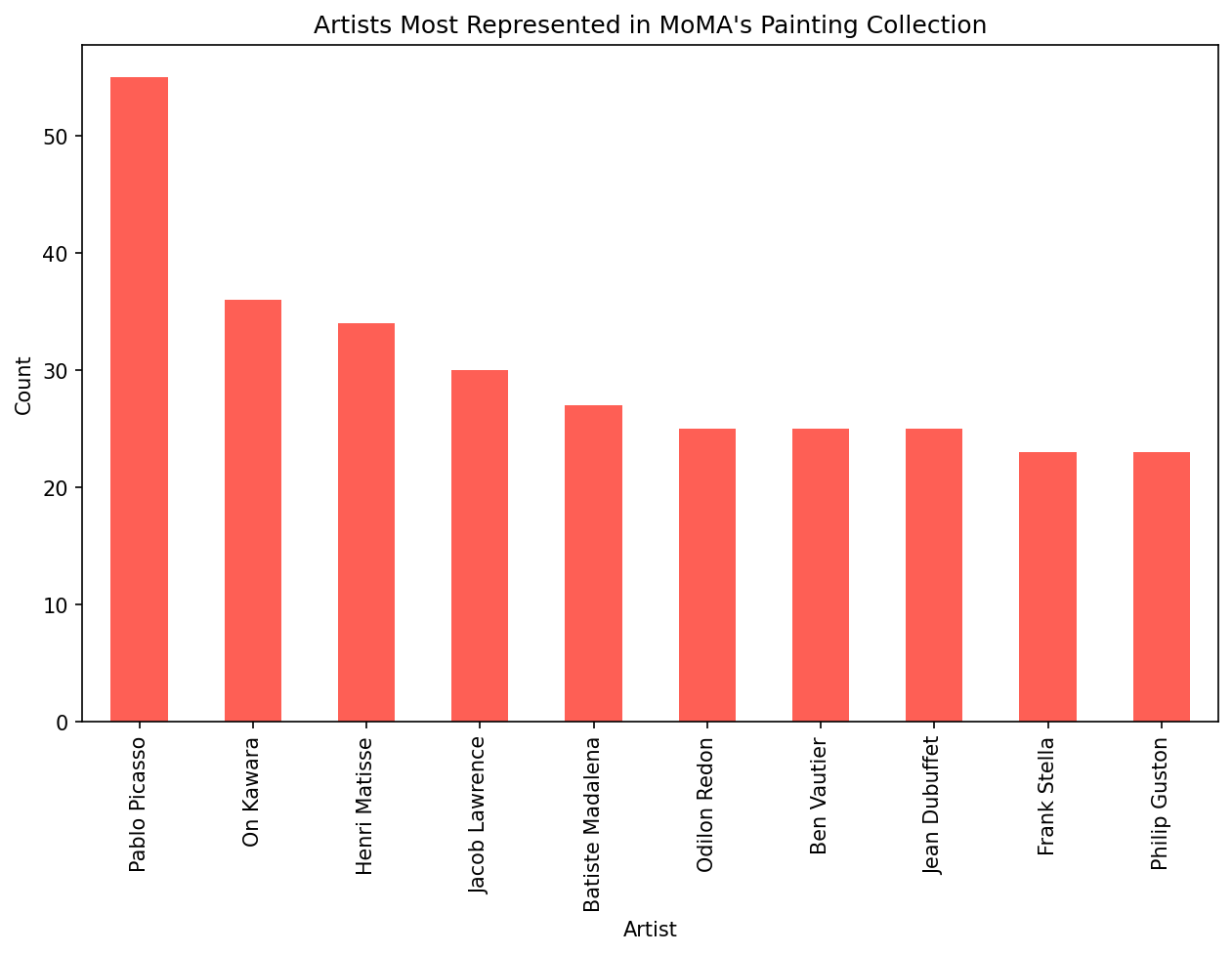
Mode for Categorical Variables
Last of all we have the mode, which specifies the most frequently occuring value. This is meaningless in the context of quantitative variables such as that which we’ve been looking at here. Does it really tell us anything to know what the most frequently occurring age of an artwork is? Probably not much.
It’s more common to use the mode with categorical variables. For instance, if we wanted to see which artist was most represented amongst MoMA’s painting collection, that is the mode. In this case, it’s Picasso, with 55 paintings at MoMA–he’s the most represented artist and thus most representative of the collection according to this measure of central tendency.