
Art Stats Illustrated: Measures of Variability
In this series of posts, I illustrate the fundamental stats concepts I'm teaching myself with art-related datasets.
What’s Variability?
The various measures of central tendency that I reviewed last time give us a sense of a “typical” value for a set of numbers (although, as we saw, some measures may be more or less typical than others). While metrics like mean or media provide useful information, however, they only tell part of the story.
What’s missing from such summary statistics is any sense of how spread out the values are. Let’s look at two examples to illustrate what I mean
# Import numpy
import numpy as np

# Set random seed
rs = np.random.RandomState(123)

# Create array of 20 random integers from 90 to 110, inclusive
arr1 = rs.randint(90, 111, 20)

# Create array of 20 random integers from 0 to 200, inclusive
arr2 = rs.randint(0, 201, 20)

print('arr1: {}'.format(arr1))
print('-> Mean: {}'.format(arr1.mean()))
print()
print('arr2: {}'.format(arr2))
print('-> Mean: {}'.format(arr2.mean()))
arr1: [103  92  92  96 107 109 100  91  90 107 105  99  90 104  90 105 109 104
  94  90]
-> Mean: 98.85

arr2: [ 68  49  55 195   2  84  39  66  84  47 189 176 135 105  99 124  92 180
 102  97]
-> Mean: 99.4
Above I’ve created two array of 20 random integers each, the first comprising numbers from 90 to 110 inclusive and the second comprising numbers from 0 to 200 inclusive. Both share a similar mean-98.85 and 99.4. But these nearly identical numbers provide no insight whatsoever into the fact that the spread in the latter group is far greater than that of the former.
This is where measures of variability come in, which give us a way of quantifying the amount of spread. There are a few basic measures of variability:
- Range (maximum value - minimum value): While subtracting the minimum value from the maximum value gives us the full range in which values occur, this number can be misleading, since it is extremely susceptible to outliers.
- Intquartile Range (IQR): Here we subtract not the minumum value from the maximum value, but the value at the 25th percentile from the value at the 75th percentile, which gives us the range where the middle 50% of values occur. This is a more robust solution, since it is not vulernable to extreme values in either direction.
- Standard Deviation: The average distance of each value from the mean. If the standard deviation is relatively small, it means that, on average, each value is not very far from the mean. A large standard deviation on the other hand means that, on average, the values are quite far from the mean indeed.
I’ll illustrate each of these with The Museum of Modern Art (MoMA) Collection Dataset that I used last time.
Here’s the DataFrame we’ll be using, which includes all the works classified as paintings.
| Title | Artist | ConstituentID | ArtistBio | Nationality | BeginDate | EndDate | Gender | Date | Medium | ... | year_acquired | date_stripped | begun_year | completed_year | birth_year | death_year | artwork_age | living | artist_age | years_posthumous | |
|---|---|---|---|---|---|---|---|---|---|---|---|---|---|---|---|---|---|---|---|---|---|
| 32097 | Rope and People, I | Joan Miró | 4016 | (Spanish, 1893–1983) | (Spanish) | (1893) | (1983) | Male | Barcelona, March 27, 1935 | Oil on cardboard mounted on wood, with coil of... | ... | 1936.0 | 1935 | 1935.0 | 1935.0 | 1893.0 | 1983.0 | 1.0 | 1 | 43.0 | NaN |
| 33171 | Fire in the Evening | Paul Klee | 3130 | (German, born Switzerland. 1879–1940) | (German) | (1879) | (1940) | Male | 1929 | Oil on cardboard | ... | 1970.0 | 1929 | 1929.0 | 1929.0 | 1879.0 | 1940.0 | 41.0 | 0 | NaN | 30.0 |
| 33428 | Portrait of an Equilibrist | Paul Klee | 3130 | (German, born Switzerland. 1879–1940) | (German) | (1879) | (1940) | Male | 1927 | Oil and collage on cardboard over wood with pa... | ... | 1966.0 | 1927 | 1927.0 | 1927.0 | 1879.0 | 1940.0 | 39.0 | 0 | NaN | 26.0 |
| 34488 | Guitar | Pablo Picasso | 4609 | (Spanish, 1881–1973) | (Spanish) | (1881) | (1973) | Male | Paris, early 1919 | Oil, charcoal and pinned paper on canvas | ... | 1955.0 | 1919 | 1919.0 | 1919.0 | 1881.0 | 1973.0 | 36.0 | 1 | 74.0 | NaN |
| 35406 | Grandmother | Arthur Dove | 1602 | (American, 1880–1946) | (American) | (1880) | (1946) | Male | 1925 | Shingles, needlepoint, page from Concordance, ... | ... | 1939.0 | 1925 | 1925.0 | 1925.0 | 1880.0 | 1946.0 | 14.0 | 1 | 59.0 | NaN |
5 rows × 39 columns
Range
We’ll start by considering the full range of painting widths
# Compute max, min, and range
max_width = paintings['Width (cm)'].max()
min_width = paintings['Width (cm)'].min()
width_range = max_width - min_width
cm_to_ft = 0.0328084

# Print results
print("Max. painting width: {:,.2f} cm / {:,.2f} ft".format(max_width, max_width * cm_to_ft))
print("Min. painting width: {:,.2f} cm / {:,.2f} ft".format(min_width, min_width * cm_to_ft))
print("Min. painting width: {:,.2f} cm / {:,.2f} ft".format(width_range, width_range * cm_to_ft))
Max. painting width: 4,663.45 cm / 153.00 ft
Min. painting width: 4.10 cm / 0.13 ft
Min. painting width: 4,659.35 cm / 152.87 ft
So we can say that the paintings in MoMA’s collection range between about 4cm in width to nearly 46 meters! At one extreme is Barnett Newman’s The Wild (1950), a vertical line of a painting. And at the other is Jennifer Bartlett’s Rhapsody (1975-76), a huge painting installation that’s made up of 987 one-foot-square panels.
But does this really tell us much? Sure, it gives us the extremes, within which the widths of 100% of MoMA’s painting collection are contained. But it doesn’t tell us how most of the widths are dispersed. In other words, maybe Newman and Bartlett’s works are outliers, meaning that their widths are substantially different from the widths of the bulk of the paintings in MoMA’s collection.
Interquartile Range
A better option would be to look at the interquartile range–that is, the difference between the 75th and 25th percentiles. This gives us the range of the central 50% of the distribution. And because outliers, by definition, exist not at the center but at extremes, the interquartile range has the wonderful distiction of being invulnerable to them. It is a metric, we could say, that is robust.
So let’s have a look.
# Compute 1st and 3rd quartiles
q1 = paintings['Width (cm)'].quantile(.25)
q3 = paintings['Width (cm)'].quantile(.75)
iqr = q3 - q1

# Print results
print("25th percentile (1st quantile): {:,.2f} cm / {:,.2f} ft".format(q1, q1 * cm_to_ft))
print("75th percentile (3st quantile): {:,.2f} cm / {:,.2f} ft".format(q3, q3 * cm_to_ft))
print("Interquartile Range (IQR)): {:,.2f} cm / {:,.2f} ft".format(iqr, iqr * cm_to_ft))
25th percentile (1st quantile): 60.15 cm / 1.97 ft
75th percentile (3st quantile): 167.66 cm / 5.50 ft
Interquartile Range (IQR)): 107.50 cm / 3.53 ft
This looks much more reasonable! Now we can say that the middle 50% of paintings vary between about 2 and 5.5 feet in width and thus have an interquartile range of about 3.5 feet.
We can use a histogram to visualize this.
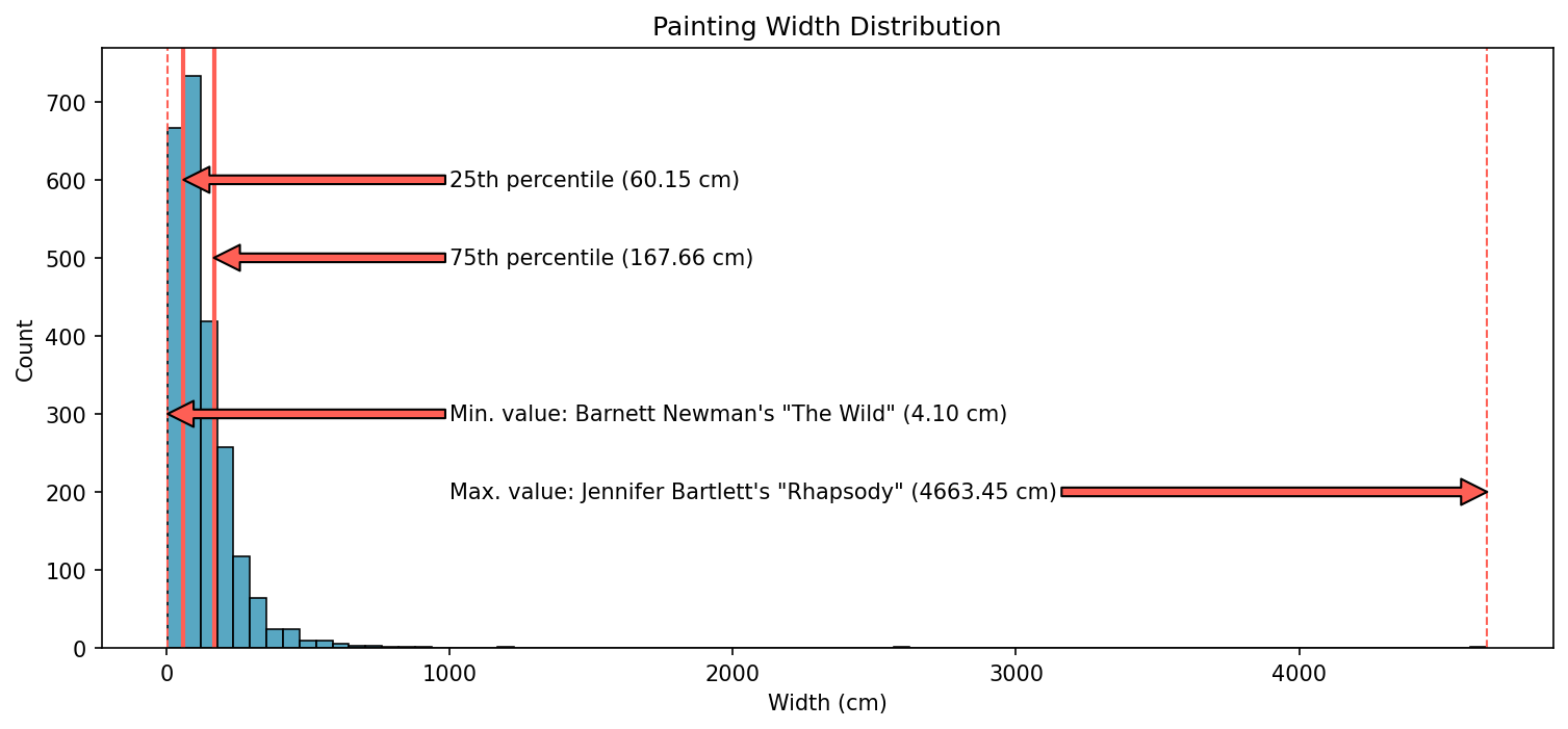
This chart makes it painfully clear just how misleading the original range calculation was, since the vast majority of paintings appear to be less than 500 cm (which makes sense, since 500 cm, or 5 m, is HUGE as it is!). In fact, this distribution is so positively skewed that the entire IQR, well, it narrow enough to be Newman’s The Wild. This makes it clear that the interquartile range is vastly superior to the full range when it comes to providing some sense of how varied the observations are.
Another way of quickly visualizing variability like this is with a boxplot.
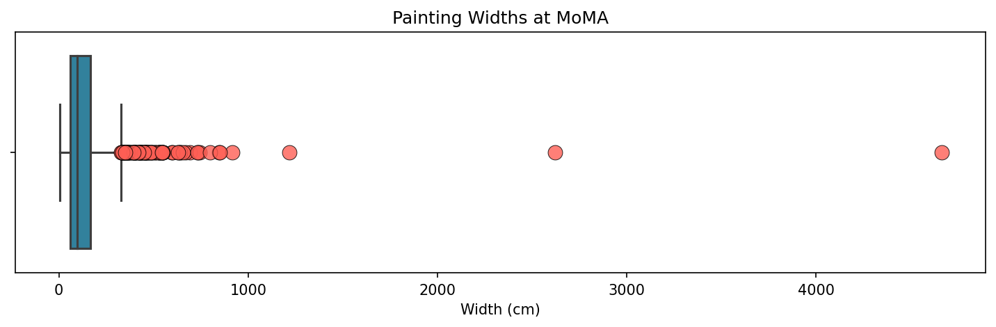
It takes a little getting used to if you haven’t looked at one of these before. The thin blue shaded are represents the interquartile range, and the vertical line in the middle is the median (50th percentile) value. The bars sticking out on either side are called whiskers, which by convention extend past the 25th and 75th percentiles by 1.5 x the IQR (in this case about 161.3 cm) in either direction. All those pink circules beyond the right whisker? Those are outliers. We can see Bartlett’s Rhapsody clearly at the right, and then James Rosenquist’s behemoth F-111 (1964-65) after that.
Sometimes it’s best to let outliers be outliers and ignore them if what we’re interested in is getting a sense of a distribution’s central tendency and variability, in which case we’d get a boxplot that looks like this:
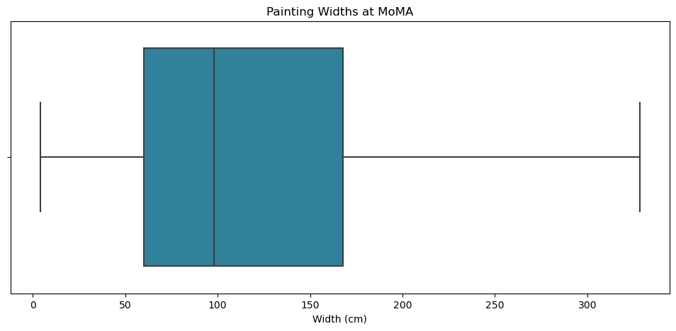
That right there gives us a damn good picture of MoMA’s painting collection when it comes to width.
Standard Deviation
The last foundational measure of variability is standard deviation, which sounds complicated but is just the average (i.e., standard) difference (i.e., deviation) of each observation from the mean. In other words, if we have a distribution with a mean of 100 and standard deviation of 5, we could say that, on average, the observations are +/- 5 from the mean.
Like the mean, standard deviation is not robust to outliers, since an outlier is very, very far from the mean and will bias the standard deviation in that direction.
# Compute mean width and st. dev.
mean_width = paintings['Width (cm)'].mean()
std_width = paintings['Width (cm)'].std()

print("Mean width: {:,.2f} cm / {:,.2f} ft".format(mean_width, mean_width * cm_to_ft))
print("Standard Deviation: {:,.2f} cm / {:,.2f} ft".format(std_width, std_width * cm_to_ft))
Mean width: 130.94 cm / 4.30 ft
Standard Deviation: 150.58 cm / 4.94 ft
To wrap this in english, we’d say that the mean painting width if 4.3 feet with a standar deviation of almost 5 feet, meaning that, on average, paintings are 4.3 ft. +/- 5 ft.
Let’s compare that to our robust measures–median and IQR.
median_width = paintings['Width (cm)'].median()

print("Median width: {:,.2f} cm / {:,.2f} ft".format(median_width, median_width * cm_to_ft))
print("IQR: {:,.2f} cm / {:,.2f} ft".format(iqr, iqr * cm_to_ft))
Median width: 98.05 cm / 3.22 ft
IQR: 107.50 cm / 3.53 ft
We can definitely see how Bartlett’s and Rosenquist’s (and others’) gargantuan works are biasing the mean and standard deviation in the positive direction. These measures are suggesting that what’s “typical” at MoMA are bigger and more varied that what’s actually true.
The advantage of mean and standard deviation, however, is that they take into account the entire spectrum of observations, which, as we’ve seen, is not the case with median and interquartile range. If a distribution was more symmetrical, the former metrics would thus provide a more accurate and comprehensive estimation.
As one final example, let’s revisit the more symmetrical distribution of painter’s ages at the time of acquisition (for painters still living at that event).
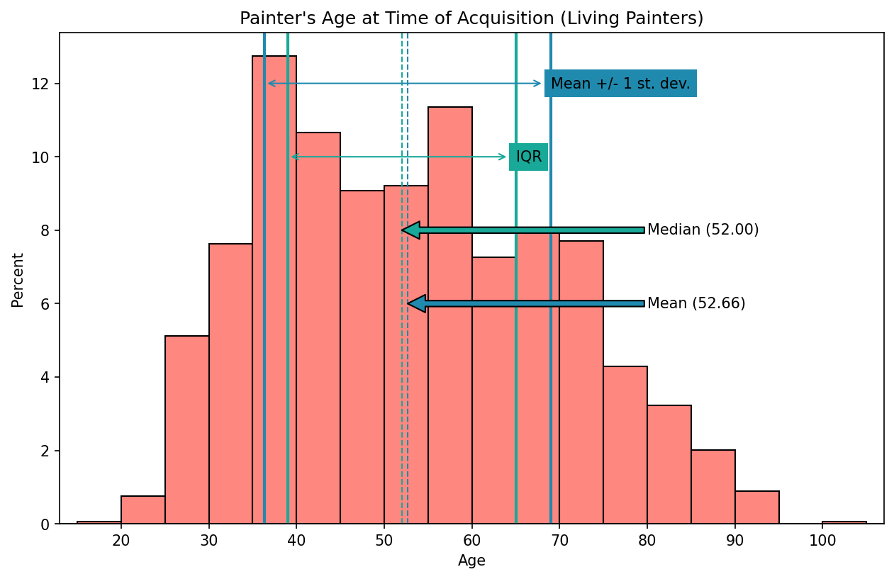
Given that this distribution is much more symmetrical, my feeling is that the mean (rather than median) would offer a more accurate representation of its central tendency as would the standard deviation (rather than IQR) for representing its variability.